 FigureCheck
How to linearize experimental data without misleading yourself
Use logarithms and reciprocal transformations to test physical relationships while checking assumptions and residuals.
Linearization transforms a proposed model into a straight-line form. Choose the transformation from scientific theory, fit and inspect the transformed relationship, and remember that transformed residuals and uncertainties do not behave like those on the original scale.
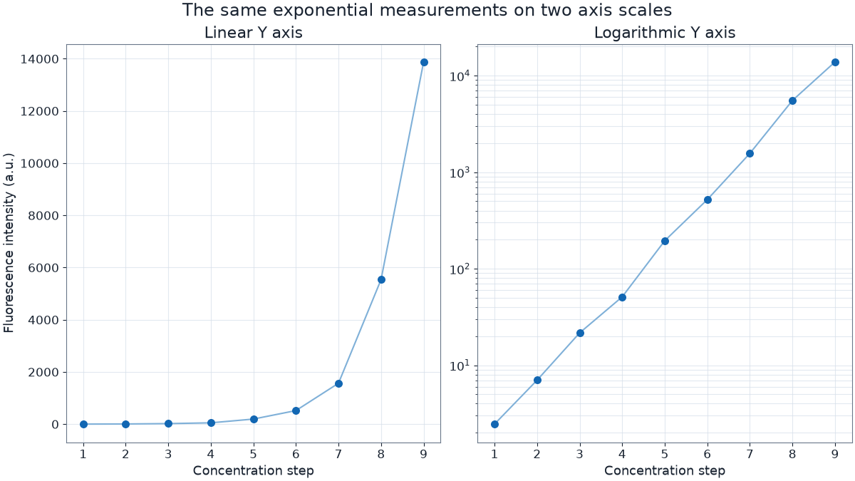
Start from a model, not a desired straight line
For y = A exp(kx), plotting ln(y) against x gives slope k and intercept ln(A). For y = A x to the power n, plotting ln(y) against ln(x) gives slope n. Reciprocal forms can linearize some inverse relationships. Values outside a transform's domain must be handled scientifically, not silently discarded.
Check the original scale too
A line that looks convincing after transformation can still fit poorly where the original response matters most. Compare residuals, uncertainty, and predictions on the original scale. If measurement errors are additive on the original scale, a log transform changes their structure and may require a different fitting method.
Worked example: testing a power law
Suppose theory proposes y = A x^n and all values are positive. Plot log(y) against log(x). A linear gradient of 1.8 estimates n = 1.8, while the intercept estimates A after reversing the logarithm. Then graph the resulting power-law curve against the untransformed data and inspect residuals.
Common mistakes to avoid
- Taking logarithms of zero or negative values
- Choosing a transform only because it raises R-squared
- Reporting transformed coefficients without converting them back
Open an editable example and apply the idea to a real graph.
Sources and further reading
These links support the scientific principles summarized above. Always follow the reporting rules required by your course, laboratory, journal, or field.