Cubic spline curve fitting: knots, smoothness, and when to use it

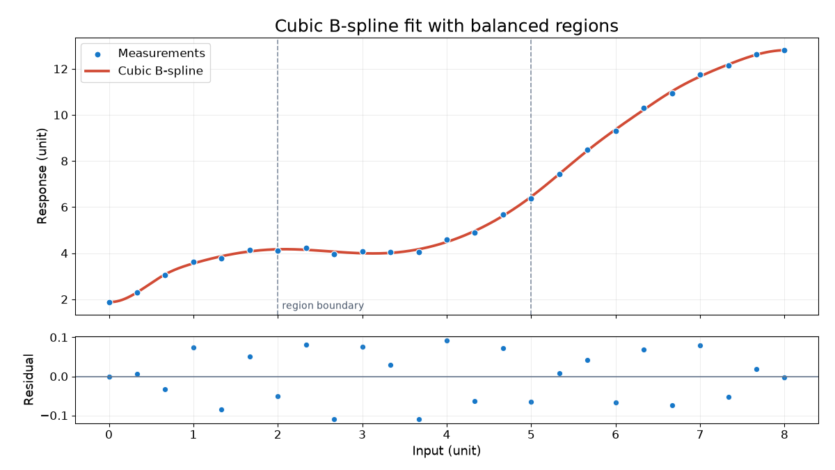
What is a cubic spline fit?

A cubic spline represents one smooth curve using several local cubic polynomial pieces. The locations where the pieces meet are called knots. A cubic B-spline is a numerically stable basis for calculating that curve; it is not a sequence of unrelated trend lines.

FigureCheck keeps the fitted spline continuous through its internal knots, including continuous first and second derivatives. This avoids visible corners while allowing different parts of the X range to have different curvature.

When should you use a cubic spline?

• Use one when the relationship is smooth but no simple physical equation describes the full shape.
• Use one for interpolation or descriptive trend display inside the measured X range.
• Consider one when a global polynomial bends badly at the ends or needs an unjustifiably high degree.
• Do not treat the spline as a physical law merely because it follows the observations closely.

A spline is usually weak for extrapolation. Outside the measured range, its shape is driven by mathematical continuation rather than new evidence.

How to choose spline region boundaries

FigureCheck accepts ordered X values as region boundaries. The first and last values define the fitted span. Interior values tell the fitter where short and long sections should receive balanced attention; FigureCheck then adds internal B-spline support where the data density requires it.

1. Begin with automatic regions or a small number of scientifically meaningful boundaries.
2. Add a boundary near a real change in curvature or sampling density, not beside every noisy point.
3. Inspect the residual plot and the curve near every boundary.
4. Compare with a simpler fit and ask whether the extra flexibility improves validation behavior.

More knots can reduce training residuals while increasing sensitivity to noise. A close visual fit is not automatically a reliable predictive model.

Spline fitting versus polynomial regression

A polynomial fit is global: changing one coefficient affects the curve across the entire domain. A spline is local: an additional knot mainly changes nearby behavior. This often makes splines more stable for complicated shapes, but the coefficients are less convenient as one compact scientific equation.

Use the polynomial degree guide to compare both approaches, then read how to interpret residuals.

How to report a spline responsibly

State the spline degree, fitting span, how boundaries or knots were chosen, whether uncertainty weights were used, and whether the purpose was interpolation, smoothing, or prediction. Preserve the generated Python code so another person can reproduce the curve.

For the underlying implementation, see the official SciPy B-spline documentation.